Response surface models
Response surface models, also known as surrogate models or metamodels, can be used to develop a fast-running approximation to an expensive simulation. para-atm provides the ResponseSurface base class to define general functionality that can be shared across different response surface implementations. A Gaussian process regression capability, powered by scikit-learn, is provided by the SklearnGPRegressor class. Additional response surface model types may be added in the future.
To get started immediately, refer to the Examples section.
Response surface base class
-
class
paraatm.rsm.base.ResponseSurface(X, Y)¶ Base class for response surface models
Derived classes should:
- Implement an __init__ method that fits the model and calls super().__init__
- Implement a __call__ method for making predictions. See
paraatm.rsm.gp.SklearnGPRegressor.__call__().
-
plot(ax=None, lb=None, ub=None, range_factor=1.1, ci=True, show_data=True, input_vals=None, ivar=None, color=None, legend=True, ncol_leg=3)¶ Create 1D response surface plots
By default, plot 1D curves of all variables on the same graph, but can also plot individual curves or subsets.
Parameters: - ax (matplotlib.axes or None) – Axis to plot on. If None, create new axis.
- lb (float) – Lower bound, only supported for single-variable plot
- ub (float) – Upper bound, only supported for single-variable plot
- range_factor (float) – Factor used to determine default plotting range. The plotting range is determined as a multiple of the data range.
- ci (bool) – Whether or not to plot confidence intervals for 1-D plots
- show_data (bool) – Whether to plot the training data. For slice plots, training data are projected
- input_vals (array) – Values to use for non-varying inputs (default to mean of training data)
- ivar (int or list of ints) – Variable index to plot. Can be scalar or a list. Default is to plot all variables.
- color (str) – Plotting color, for single-variable plots only
- legend (bool) – Whether to include legend
- ncol_leg (int) – Number of columns to use for formatting legend
-
surface_plot(ax=None, lb=None, ub=None, range_factor=1.1, ngrid=40, show_data=True, input_vals=None, slice_vars=None, surf_args=None)¶ Create 2D surface plot
Parameters: - ax (matplotlib.axes or None) – Axis to plot on. If None, create new axis
- lb (array) – Lower bound to use for each variable
- ub (array) – Upper bound to use for each variable
- range_factor (float) – Factor used to determine default plotting range. The plotting range is determined as a multiple of the data range.
- ngrid (int) – Grid density used in each dimension
- show_data (bool) – Whether to plot training data
- input_vals (array) – Array of input values, required when plotting a slice of a surface with more than two input variables.
- slice_vars (tuple) – Length-2 tuple with indices of the variables to plot. Required when the response surface has more than two input variables.
- surf_args (dict) – Additional keyword arguments to send to Axes3D.plot_surface
Returns: Return type: matplotlib.axes
Gaussian process regression
-
class
paraatm.rsm.gp.SklearnGPRegressor(X, Y, noise=False, n_restarts_optimizer=10, alpha=1e-10, kernel=None, optimizer='fmin_l_bfgs_b')¶ Gaussian Process regression using scikit-learn
-
__init__(X, Y, noise=False, n_restarts_optimizer=10, alpha=1e-10, kernel=None, optimizer='fmin_l_bfgs_b')¶ Create GP regression instance and fit to training data
Parameters: - X (array) – 2d array of input values, with each row representing a case and each column a variable
- Y (array) – 1d array of output values
- noise (bool) – Whether the outputs are observed with noise. If True, the noise variance is estimated as part of the fitting. Additionally, scikit-learn includes the noise in the prediction standard deviation.
- n_restarts_optimizer (int) – Number of times optimizer is restarted using randomly selected initial points
- alpha (float) – Value added to diagonal of covariance matrix during fitting. Unlike the noise variance that can be fit through the WhiteKernel, the alpha value is not included in the predicted standard deviation.
- kernel (kernel object) – Kernel specifying the covariance function of the GP. If None, RBF (a.k.a., squared exponential) is used with unique length parameters for each dimension.
- optimizer (str, callable, or None) – Passed on to sklearn. In particular, None can be used to fix the kernel parameters instead of optimizing them.
-
__call__(X, return_stdev=False)¶ Compute predicted mean and standard deviation (optionally) at specified input(s)
Parameters: - X (array, 1d or 2d) – Input values, either as a single point (1d array) or a 2d array containing a set of points
- return_stdev (bool) – Whether to return standard deviation of the prediction, in addition to the mean.
Returns: The return value is either a tuple containing the mean and standard deviation (if return_stdev==True) or the mean value only. If ndim(X)==2, then the mean and standard deviations are returned as arrays, otherwise they are floats.
Return type: tuple, float, or array
-
fit_rsquared()¶ Get fit R-squared value
-
loo_rsquared()¶ Get leave-one-out R-squared value
Kernel parameters and normalization constants are not changed. The intent is to test holding out the observations but not re-fitting the kernel parameters.
-
Examples
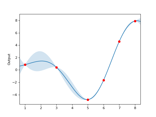
Here is an example showing a GP fit to a 1D function, with confidence bounds:
import matplotlib.pyplot as plt
import numpy as np
from paraatm.rsm.gp import SklearnGPRegressor

X = np.array([1., 3., 5., 6., 7., 8.])
Y = X * np.sin(X)
X = X[:,np.newaxis] # Make input array 2d

# Use n_restarts_optimizer=0 to get reproducible behavior
gp = SklearnGPRegressor(X, Y, n_restarts_optimizer=0)

gp.plot()

plt.show()
(Source code, png, hires.png, pdf)
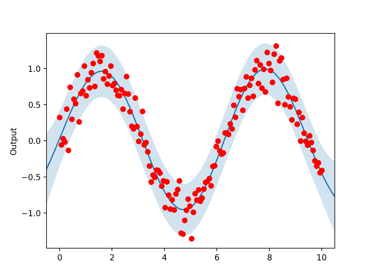
The Gaussian Process model can also accommodate noisy data, as shown in the below example:
import matplotlib.pyplot as plt
import numpy as np
from paraatm.rsm.gp import SklearnGPRegressor

ndata = 150
np.random.seed(1)
X = np.linspace(0,10,ndata)
Y = np.sin(X) + np.random.normal(0,.2, size=ndata)
X = X[:,np.newaxis]

gp = SklearnGPRegressor(X, Y, n_restarts_optimizer=0, noise=True)

gp.plot()

plt.show()
(Source code, png, hires.png, pdf)

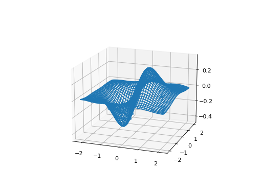
And an example of a 2D function, using surface_plot():
import matplotlib.pyplot as plt
import numpy as np
from paraatm.rsm.gp import SklearnGPRegressor

np.random.seed(1)
X = np.random.uniform(-2, 2, size=(30,2))
Y = X[:,0] * np.exp(-X[:,0]**2 - X[:,1]**2)

gp = SklearnGPRegressor(X, Y, n_restarts_optimizer=0)

ax = gp.surface_plot()
ax.view_init(17, -70)

plt.show()
(Source code, png, hires.png, pdf)